Introduction to Flexible Clustering of (Mixed-With-)Ordinal Data • flexord

Package description and contents

Package flexord is an add on-package to packages flexclust and flexmix that provide suites for partitioning and model-based clustering with flexible method switching and comparison.

We provide additional distance and centroid calculation functions, and additional model drivers for component distributions that are tailored towards ordinal, or mixed-with-ordinal data. These new methods can easily be plugged into the capabilities for clustering provided by flexclust and flexmix.

By plugging them into the flex-scheme, they can be used for:

one-off K-centroids and model-based clustering (via flexclust::kcca and flexmix::flexmix),
repeated clustering runs with various cluster numbers k (via flexclust::stepFlexclust and flexmix::stepFlexmix),
bootstrapping repeated clustering runs with various cluster numbers k for K-centroids clustering (via flexclust::bootFlexclust),
applying the various methods for the resulting objects, such as predict, plot, barchart, …

The new methods provided are:

Clustering Type	Function Type	Function Name	Method	Scale Assumptions	NA Handling	Source
Partitioning (K-centroids)	distance	`distSimMatch`	Simple Matching Distance	nominal	not implemented	Kaufman and Rousseeuw (1990), p. 19
		`distGDM2`	GDM2 distance for ordinal data	ordinal	not implemented	Walesiak and Dudek (2010); Ernst et al. (2025)
		`distGower`	Gower’s distance	mixed-with-ordinal	upweighing of present variables	Kaufman and Rousseeuw (1990), p. 32-37
	centroid	`centMode`	Mode as centroid	nominal	not implemented	Weihs et al. (2005); Leisch (2006)
		`centMin`	Factor level with minimal distance as centroid	nominal/ordinal	not implemented	Ernst et al. (2025)
		`centOptimNA`	Centroid calculation by general purpose optimizer	numeric	complete-case analysis	Leisch (2006)
	wrapper	`kccaExtendedFamily`	Creates a `kccaFamily` object pre-configured for kModes-, kGDM2- or kGower clustering
Model-based	driver	`FLXMCregnorm`	Regularized multivariate normal distribution	numeric	not implemented	Fraley and Raftery (2007); Ernst et al. (2025)
		`FLXMCregmultinom`	Regularized multivariate multinomial distribution	nominal	not implemented	Galindo Garre and Vermunt (2006); Ernst et al. (2025)
		`FLXMCregbinom`	Regularized multivariate binomial distribution	ordinal	not implemented	Ernst et al. (2025)
		`FLXMCbetabinomial`	Regularized multivariate beta-binomial distribution	ordinal	not implemented	Kondofersky (2008); Ernst et al. (2025)

Example 1: Clustering purely nominal data

We load necessary packages and set a random seed for reproducibility.

library("flexord")
library("flexclust")
library("flexmix")
set.seed(1111)

As an example for purely nominal data, we will use the classic Titanic data set:

titanic_df <- data.frame(Titanic)
titanic_df <- titanic_df[rep(1:nrow(titanic_df), titanic_df$Freq), -5]
str(titanic_df)
#> 'data.frame':    2201 obs. of  4 variables:
#>  $ Class   : Factor w/ 4 levels "1st","2nd","3rd",..: 3 3 3 3 3 3 3 3 3 3 ...
#>  $ Sex     : Factor w/ 2 levels "Male","Female": 1 1 1 1 1 1 1 1 1 1 ...
#>  $ Age     : Factor w/ 2 levels "Child","Adult": 1 1 1 1 1 1 1 1 1 1 ...
#>  $ Survived: Factor w/ 2 levels "No","Yes": 1 1 1 1 1 1 1 1 1 1 ...

Partitioning approach

We can conduct K-centroids clustering with the kModes algorithm directly on the data frame¹:

kcca(titanic_df, k = 4, family = kccaExtendedFamily('kModes'))
#> kcca object of family 'kModes' 
#> 
#> call:
#> kcca(x = titanic_df, k = 4, family = kccaExtendedFamily("kModes"))
#> 
#> cluster sizes:
#> 
#>    1    2    3    4 
#>  140  396  287 1378

Let us assume that for some reason we are unhappy with the mode as a centroid, and rather want to use an optimized centroid value, by choosing the factor level for which Simple Matching distance² is minimal:

kcca(titanic_df, k = 4,
     family = kccaFamily(dist = distSimMatch, 
                         cent = \(y) centMin(y, dist = distSimMatch,
                                             xrange = 'columnwise')))
#> kcca object of family 'distSimMatch' 
#> 
#> call:
#> kcca(x = titanic_df, k = 4, family = kccaFamily(dist = distSimMatch, 
#>     cent = function(y) centMin(y, dist = distSimMatch, xrange = "columnwise")))
#> 
#> cluster sizes:
#> 
#>   1   2   3   4 
#> 369 737 317 778

This already showcases one of the advantages of package flexclust: As the name suggests, we are quickly able to mix and match our distance and centroid functions, and quickly create our own K-centroids algorithms.

Furthermore, flexclust allows us to decrease the influence of randomness via running the algorithm several times, and keeping only the solution with the minimum within cluster distance. This can be done for one specific number of clusters k or several values k:

stepFlexclust(data.matrix(titanic_df), k = 2:4, nrep = 3, 
              family = kccaExtendedFamily('kModes')) 
#> 2 : * * *
#> 3 : * * *
#> 4 : * * *
#> stepFlexclust object of family 'kModes' 
#> 
#> call:
#> stepFlexclust(x = data.matrix(titanic_df), k = 2:4, nrep = 3, 
#>     family = kccaExtendedFamily("kModes"))
#> 
#>   iter converged distsum
#> 1   NA        NA  651.50
#> 2  200     FALSE  413.50
#> 3  200     FALSE  278.75
#> 4  200     FALSE  246.00

The output above shows the solutions with lowest within cluster distance out of 3 runs for 2 to 4 clusters, in comparison to 1 big cluster. However, none of the algorithms converged. Presumably this is due to observations which have the same distance to two centroids and which are randomly assigned to one of the two centroids, implying that the partitions are still changing in each iteration, even if the centroids do not change.

Selecting a suitable number of clusters based on the output of stepFlexclust might be still difficult. This is where bootFlexclust comes in. In bootFlexclust, nboot bootstrap samples of the original data are drawn, on which stepFlexclust is performed for each k. This results in k $\times$ nboot best out of nrep clustering solutions obtained for each bootstrap data set. Based on these solutions cluster memberships are predicted for the original data set, and the stability of these partitions is tested via the Adjusted Rand Index (Hubert and Arabie 1985):

(nom <- bootFlexclust(data.matrix(titanic_df),
                      k = 2:4, nrep = 3, nboot = 5, 
                      family = kccaExtendedFamily('kModes')))
#> An object of class 'bootFlexclust' 
#> 
#> Call:
#> bootFlexclust(x = data.matrix(titanic_df), k = 2:4, nboot = 5, 
#>     nrep = 3, family = kccaExtendedFamily("kModes"))
#> 
#> Number of bootstrap pairs: 5

Note that ridiculously few repetitions are used for the sake of having a short run time.

The resulting ARIs can be quickly visualized via a predefined plotting method:

plot(nom)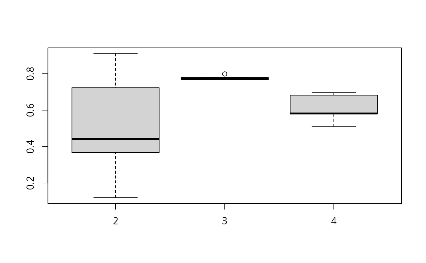

Our plot indicates that out of the 2 to 4 cluster solutions, a three cluster solution has the highest median ARI out of 5 runs.

Now, after deciding on a suitable cluster number, we could select the corresponding cluster solution from kcca or stepFlexclust, and make use of the further visualization, prediction, and other tools. For this, we refer to the documentation available in Leisch (2006) and Dolnicar, Grün, and Leisch (2018).

Model-based approach

We also offer an algorithm specifically designed for model-based clustering of unordered categorical data via a regularized multinomial distribution. The multinomial driver also supports varying number of categories between variables. Then we call flexmix with a model driver specifying the number of categories:

titanic_ncats = apply(data.matrix(titanic_df), 2, max)
flexmix(formula = data.matrix(titanic_df) ~ 1, k = 3,
        model = FLXMCregmultinom(r = titanic_ncats)) 
#> 
#> Call:
#> flexmix(formula = data.matrix(titanic_df) ~ 1, k = 3, model = FLXMCregmultinom(r = titanic_ncats))
#> 
#> Cluster sizes:
#>    1    2    3 
#> 1208  364  629 
#> 
#> convergence after 125 iterations

As we have to estimate many category probabilities across multiple clusters some of those may become numerically zero. To avoid this we may use the regularization parameter $\alpha$ , which acts if we added $\alpha$ observations according to the population mean to each component:

flexmix(data.matrix(titanic_df) ~ 1, k = 3,
        model=FLXMCregmultinom(r = titanic_ncats, alpha = 1))
#> 
#> Call:
#> flexmix(formula = data.matrix(titanic_df) ~ 1, k = 3, model = FLXMCregmultinom(r = titanic_ncats, 
#>     alpha = 1))
#> 
#> Cluster sizes:
#>    1    2    3 
#>  364  629 1208 
#> 
#> convergence after 56 iterations

flexmix also offers a step method, where the EM algorithm for each k is restarted nrep times, and only the maximum likelihood solution is retained:

(nom <- stepFlexmix(data.matrix(titanic_df)~1, k = 2:4,
                    nrep = 3, #please increase for real-life use
                    model = FLXMCregmultinom(r = titanic_ncats)))
#> 2 : * * *
#> 3 : * * *
#> 4 : * * *
#> 
#> Call:
#> stepFlexmix(data.matrix(titanic_df) ~ 1, model = FLXMCregmultinom(r = titanic_ncats), 
#>     k = 2:4, nrep = 3)
#> 
#>   iter converged k k0    logLik      AIC      BIC      ICL
#> 2   38      TRUE 2  2 -5327.340 10680.68 10754.74 10986.90
#> 3  103      TRUE 3  3 -5202.816 10445.63 10559.57 11036.09
#> 4  121      TRUE 4  4 -5176.038 10406.08 10559.89 11454.98

The output of this is the best out of three clusterings for 3 different values of k. We are also already provided with different model selection criteria, namely, AIC, BIC and ICL.

Similar to package flexclust in the partitioning case, package flexmix also offers various plotting methods for the returned objects. We just showcase one here for simplicity:

plot(nom)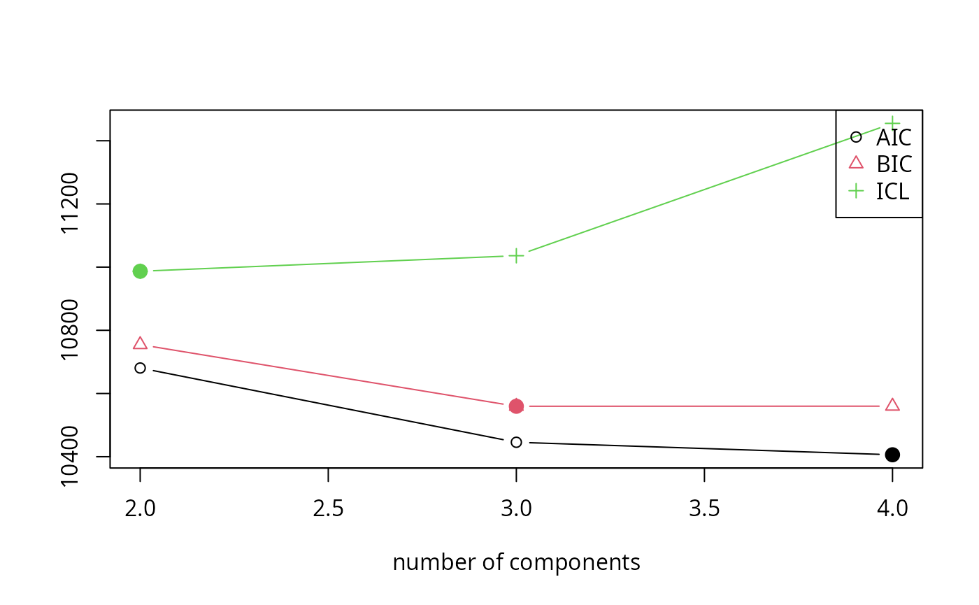

For more information on the further methods and utilities offered, check out the documentation for flexmix (browseVignettes('flexmix')).

Example 2: Clustering purely ordinal data

Our next example data set is from a survey conducted among 563 Australians in 2015 where they indicated on a scale from 1-5 how inclined they are to take 6 types of risks. It consists of purely ordinal variables without missing values, and the response level length is the same for all variables.

data("risk", package = "flexord")
str(risk)
#>  int [1:563, 1:6] 3 1 2 1 5 5 1 5 1 3 ...
#>  - attr(*, "dimnames")=List of 2
#>   ..$ : NULL
#>   ..$ : chr [1:6] "Recreational" "Health" "Career" "Financial" ...
colnames(risk)
#> [1] "Recreational" "Health"       "Career"       "Financial"    "Safety"      
#> [6] "Social"

Partitioning approach

In our package, we offer two partitioning methods designed for ordinal data: Firstly, we can apply Gower’s distance from distGower to purely ordinal data, which results in using Manhattan distance (as provided also in flexclust::distManhattan) with previous scaling as described by Kaufman and Rousseeuw (1990) and Gower’s upweighing of non-missing values:

kcca(risk, k = 4, family = kccaExtendedFamily('kGower'))
#> kcca object of family 'kGower' 
#> 
#> call:
#> kcca(x = risk, k = 4, family = kccaExtendedFamily("kGower"))
#> 
#> cluster sizes:
#> 
#>   1   2   3   4 
#> 133 123 106 201

The default centroid for this family is the general purpose optimizer centOptimNA, which is the general purpose optimizer flexclust::centOptim, just with NA removal. In our case of purely ordinal data with no missing values, we could also choose the median as a centroid:

kcca(risk, k = 4,
     family = kccaExtendedFamily('kGower', cent = centMedian))
#> kcca object of family 'kGower' 
#> 
#> call:
#> kcca(x = risk, k = 4, family = kccaExtendedFamily("kGower", cent = centMedian))
#> 
#> cluster sizes:
#> 
#>   1   2   3   4 
#> 300  65  90 108

This results in kMedians with previous scaling, and non-missing value upweighing³. In our risk example with no NAs and equal level lengths for all variables, flexclust::kccaFamily('kmedians') would suffice, but there are still many data situations where the kGower approach will be preferable.

As a second alternative designed specifically for ordinal data without missing values, we implement the GDM2 distance for ordinal data by Walesiak and Dudek (2010), which conduct only relational operations on ordinal variables. We have reformulated it for use in K-centroids analysis in Ernst et al. (2025), and implemented it in the package:

kcca(risk, k = 3, family = kccaExtendedFamily('kGDM2'))
#> kcca object of family 'kGDM2' 
#> 
#> call:
#> kcca(x = risk, k = 3, family = kccaExtendedFamily("kGDM2"))
#> 
#> cluster sizes:
#> 
#>   1   2   3 
#> 101  77 385

Same as in kGower, a default general optimizer centroid is applied, which we could replace as desired.

Another parameter used in both kGower and kGDM2 is xrange. Both algorithms require information on the range of the data object for data preprocessing, one for scaling, the other for transforming the data to empirical distributions. The range calculation can be influenced in the following ways: We can use the range of the whole x (argument all, the default for kGDM2), columnwise ranges (xrange=columnwise), a vector specifying the range of the data set, or a list of length ncol(x) with range vectors for each column. Let us assume that the highest possible response to the risk questions was Extremely often (6), but it was never chosen by any of the respondents. We can take the new assumed full range of the data into account:

kcca(risk, k = 3,
     family = kccaExtendedFamily('kGDM2', xrange = c(1, 6)))
#> kcca object of family 'kGDM2' 
#> 
#> call:
#> kcca(x = risk, k = 3, family = kccaExtendedFamily("kGDM2", xrange = c(1, 
#>     6)))
#> 
#> cluster sizes:
#> 
#>   1   2   3 
#>  97  43 423

Again, the distances, centroids, and wrapper alternatives presented can be used also in the further capabilities of flexclust.

Model-based approach

We also offer drivers for two distributions for ordinal data, which are the binomial distribution and its extension the beta-binomial distribution:

flexmix(risk~1, k=3, model=FLXMCregbinom(size=5))
#> 
#> Call:
#> flexmix(formula = risk ~ 1, k = 3, model = FLXMCregbinom(size = 5))
#> 
#> Cluster sizes:
#>   1   2   3 
#> 284  28 251 
#> 
#> convergence after 58 iterations
flexmix(risk~1, k=3, model=FLXMCregbetabinom(size=5, alpha=1))
#> 
#> Call:
#> flexmix(formula = risk ~ 1, k = 3, model = FLXMCregbetabinom(size = 5, 
#>     alpha = 1))
#> 
#> Cluster sizes:
#>   1   2   3 
#> 271  36 256 
#> 
#> convergence after 56 iterations

In both cases we specify the number of trials of the binomial distribution (size). For both distributions we can also use a regularization parameter alpha that draws the component estimates towards the population mean. While this incurs small distortions it can be helpful to avoid boundary estimates.

The beta-binomial distribution is parameterized by two parameters a and b and is therefore more flexible than the binomial. It may potentially perform better in more difficult clustering scenarios even if we assume the original data was drawn from a binomial mixture (Ernst et al. (2025)). Your mileage may vary.

We can further use the capabilities of stepFlexmix and the corresponding plot functions. See Example 1.

Treating the data as purely nominal

Treating ordered categorical data as unordered is a frequent approach. In fact, in our simulation study it was a quite competitive approach for model-based methods. However, applying kmodes to ordered data brought subpar results in the partitioning ambit (Ernst et al. 2025). For How-Tos, please look at Example 1.

Treating the data as equidistant (=integer)

Also treating ordered categorical data as integer values is at least as common as nominalization. In fact, some of the methods presented above, such as kGower - as used above on purely ordinal data without missing values - make only lax concessions towards ordinality. Depending on data characteristics and method group applied, this approach may also be a very good choice (Ernst et al. 2025).

We do not offer any new methods for this in the partitioning ambit, as already many options are available in flexclust.

In the model-based ambit we offer additional capabilities via FLXMCregnorm, which, as mentioned, is a driver for clustering with multivariate normal distributions while allowing for regularization (same as is the case for FLXMCregmultinom, regularization can help avoid degenerate solutions):

flexmix(risk ~ 1, k = 3,
        model = FLXMCregnorm(kappa_p = 0.1, #regularization parameter
                             G = 3)) #number of clusters, used for scale calculation
#> 
#> Call:
#> flexmix(formula = risk ~ 1, k = 3, model = FLXMCregnorm(kappa_p = 0.1, 
#>     G = 3))
#> 
#> Cluster sizes:
#>   1   2 
#> 505  58 
#> 
#> convergence after 43 iterations

This implements the univariate case with different variances from Fraley and Raftery (2007) . In the source paper they use an inverse gamma distribution as conjugate prior. Using the prior we can again avoid boundary estimates. Most notably the shrinkage parameter kappa_p (the suffix _p stands for prior), acts as if we added kappa_p observations according to the population mean to each component.

The scale parameter zeta_p is computed by default as the empirical variance divided by the square of the number of components. In this case we need to pass G=3. We could however specify a value for zeta_p and then omit the parameter G (we can’t have both parameter at the same time, therefore zeta_p takes precedence if both were given).

For more details see Fraley and Raftery (2007) or package Mclust.

Again, the model can be plugged into all of the further tools offered by flexmix, for some example usages see Example 1.

Example 3: Clustering mixed-type data with missing values

data("vacmot", package = "flexclust")
vacmot2 <- cbind(vacmotdesc,
                 apply(vacmot, 2, as.logical))
vacmot2 <- vacmot2[, c('Gender', 'Age', 'Income2', 'Relationship.Status', 'Vacation.Behaviour',
                       sample(colnames(vacmot), 3, replace = FALSE))]
vacmot2$Income2 <- as.ordered(vacmot2$Income2) 
str(vacmot2)
#> 'data.frame':    1000 obs. of  8 variables:
#>  $ Gender                        : Factor w/ 2 levels "Male","Female": 2 2 1 2 1 2 1 1 2 2 ...
#>  $ Age                           : num  25 31 21 18 61 63 58 41 36 56 ...
#>  $ Income2                       : Ord.factor w/ 5 levels "<30k"<"30-60k"<..: 2 5 4 2 1 2 1 2 4 2 ...
#>  $ Relationship.Status           : Factor w/ 5 levels "single","married",..: 1 2 1 1 2 2 3 4 3 2 ...
#>  $ Vacation.Behaviour            : num  2.07 2 1.23 2.17 1.72 ...
#>  $ do sports                     : logi  FALSE FALSE FALSE FALSE FALSE FALSE ...
#>  $ maintain unspoilt surroundings: logi  FALSE FALSE FALSE FALSE TRUE FALSE ...
#>  $ luxury / be spoilt            : logi  FALSE TRUE FALSE TRUE FALSE FALSE ...
colMeans(is.na(vacmot2))*100 
#>                         Gender                            Age 
#>                            0.0                            0.0 
#>                        Income2            Relationship.Status 
#>                            6.6                            0.4 
#>             Vacation.Behaviour                      do sports 
#>                            2.5                            0.0 
#> maintain unspoilt surroundings             luxury / be spoilt 
#>                            0.0                            0.0

For our last example, we chose a merged data set that is shared in flexclust. In flexclust, it is provided in the object vacmot as a $1000 \times 20$ matrix of binary responses to questions on travel motives posed to Australians in 2006, plus a separate data frame vacmotdesc with 12 demographic variables for each respondent.

This data set has been thoroughly explored for clustering in the field of market segmentation research, see for example Dolnicar and Leisch (2008). We now use it as a data example for a mixed-data case with a moderate amount of missingness. For this, we chose 1 symmetric binary variable (Gender, which was collected as Male/Female in 2006), 2 numeric variables (Age and Vacation Behaviour⁴), 1 unordered categorical variable (Relationship Status), 1 ordered categorical variable (Income2, which is a recoding of Income), and 3 randomly selected asymmmetric binary variables (3 of the 20 questions on whether a specific travel motive applies to a respondent). Missing values are present, but the percentage is low⁵.

Partitioning approach

Currently, we only offer one method for mixed-type data with missing values, which is kGower (scaling and distances as proposed by Gower (1971) and Kaufman and Rousseeuw (1990), and a general purpose optimizer centroid as provided in flexclust, but with NA omission):

kcca(vacmot2, k = 3, family = kccaExtendedFamily('kGower'))
#> kcca object of family 'kGower' 
#> 
#> call:
#> kcca(x = vacmot2, k = 3, family = kccaExtendedFamily("kGower"))
#> 
#> cluster sizes:
#> 
#>   1   2 
#> 318 682

In our example above, the default methods for each variable type are used (Simple Matching Distance for the categorically coded variables, squared Euclidean distance for the numerically/integer coded variables, Manhattan distance for ordinal variables, and Jaccard distance for logically coded variables).

We could instead provide a vector of length ncol(vacmot2) where each distance measure to be used is specified. Let us assume that we have many outliers in the variable Age, that we consider Vacation.Behaviour an ordered factor as well, and that the three binary responses to vacation motives are symmetric instead of asymmetric⁶, and for this reason want to evaluate the first with Manhattan distance, and the latter with Euclidean distance⁷:

colnames(vacmot2)
#> [1] "Gender"                         "Age"                           
#> [3] "Income2"                        "Relationship.Status"           
#> [5] "Vacation.Behaviour"             "do sports"                     
#> [7] "maintain unspoilt surroundings" "luxury / be spoilt"
xmthds <- c('distSimMatch', rep('distManhattan', 3),
            'distSimMatch', rep('distEuclidean', 3))
kcca(vacmot2, k = 3,
     family = kccaExtendedFamily('kGower', xmethods = xmthds))
#> kcca object of family 'kGower' 
#> 
#> call:
#> kcca(x = vacmot2, k = 3, family = kccaExtendedFamily("kGower", 
#>     xmethods = xmthds))
#> 
#> cluster sizes:
#> 
#>   1   2   3 
#> 276 296 428

For kGower, all numeric/integer and ordered variables are scaled as proposed by Kaufman and Rousseeuw (1990), by centering around their minimum and dividing by the range. This means that also for kGower, the range of the variables will influence the clustering results. Same as for kGDM2 (Example 2), we can specify the range to be used in parameter xrange. In the case of kGower, the default value is columnwise, where the range for each column is calculated separately.

Again, the distance, centroid and wrapper functions can be used in the further tools provided by flexclust, for examples on that see Example 1.

References

Dolnicar, Sara, Bettina Grün, and Friedrich Leisch. 2018. Market Segmentation Analysis. Management for Professionals. Singapore: Springer-Verlag. https://doi.org/10.1007/978-981-10-8818-6_2.

Dolnicar, Sara, and Friedrich Leisch. 2008. “An Investigation of Tourists’ Patterns of Obligation to Protect the Environment.” Journal of Travel Research 46 (4): 381–91. https://doi.org/10.1177/0047287507308330.

Ernst, Dominik, Lena Ortega Menjivar, Theresa Scharl, and Bettina Grün. 2025. “Ordinal Clustering with the Flex-Scheme.” Austrian Journal of Statistics.

Fraley, Chris, and Adrian E Raftery. 2007. “Bayesian Regularization for Normal Mixture Estimation and Model-Based Clustering.” Journal of Classification 24 (2): 155–81. https://doi.org/10.1007/s00357-007-0004-5.

Galindo Garre, Francisca, and Jeroen K Vermunt. 2006. “Avoiding Boundary Estimates in Latent Class Analysis by Bayesian Posterior Mode Estimation.” Behaviormetrika 33: 43–59. https://doi.org/10.2333/bhmk.33.43.

Gower, J. C. 1971. “A General Coefficient of Similarity and Some of Its Properties.” Biometrics 27 (4): 857–71. https://doi.org/10.2307/2528823.

Hubert, Lawrence, and Phipps Arabie. 1985. “Comparing Partitions.” Journal of Classification 2 (1): 193–218. https://doi.org/10.1007/BF01908075.

Kaufman, Leonard, and Peter Rousseeuw. 1990. Finding Groups in Data: An Introduction to Cluster Analysis. Wiley Series in Probability and Statistics. New York: John Wiley & Sons. https://doi.org/10.1002/9780470316801.

Kondofersky, Ivan. 2008. “Modellbasiertes Clustern Mit Der Beta-Binomialverteilung.” Bachelor's thesis.

Leisch, Friedrich. 2006. “A Toolbox for K-Centroids Cluster Analysis.” Computational Statistics & Data Analysis 51 (2): 526–44. https://doi.org/10.1016/j.csda.2005.10.006.

Walesiak, Marek, and Andrzej Dudek. 2010. “Finding Groups in Ordinal Data: An Examination of Some Clustering Procedures.” In Classification as a Tool for Research, edited by Hermann Locarek-Junge and Claus Weihs, 185–92. Berlin, Heidelberg: Springer-Verlag. https://doi.org/10.1007/978-3-642-10745-0_19.

Weihs, Claus, Uwe Ligges, Karsten Luebke, and Nils Raabe. 2005. “klaR Analyzing German Business Cycles.” In Data Analysis and Decision Support, edited by D. Baier, R. Decker, and L. Schmidt-Thieme, 335–43. Berlin: Springer-Verlag. https://doi.org/10.1007/3-540-28397-8_36.

Internally, it will be converted to a data.matrix. However, as only equality operations and frequency counts are used, this is of no consequence.↩︎
i.e., the mean disagreement count↩︎
Note to selves: Strictly, it doesn’t, as Fritz never made his centMedianNA public↩︎
Mean environmental friendly behaviour score, ranging from 1 to 5↩︎
This is by choice. While Gower’s distance is designed to handle missingness via variable weighting, and the general optimizer used here is written to omit NAs, both methods will degenerate with high percentages of missing values. While we have not yet determined the critical limit, we have successfully run the algorithm on purely ordinal data with MCAR missingness percentages of up to 30%. However, common sense dictates that solutions obtained for such high missingness percentages need to be treated with caution.↩︎
meaning that 2 disagreements are just as important as 2 agreements↩︎
we could achieve symmetric treatment also via Simple Matching Distance↩︎